
Mixed-family VAR
bvarnet allows combining different outcome families in a
single VAR model by passing a named vector to the family
argument. This is useful when the variables in the network are measured
on different scales.
In this example we fit a mixed-family VAR(1) with three types of outcome:
-
ordinal:
stress_level(5-point Likert items) -
binary:
happyornot_bin(binarised daily average) -
gaussian:
sleep_duration(hours)
Load Data
Again, we start with loading the data
data(studentlife)Priors
For a mixed-family model we specify priors for all parameter types
that can appear. Here that means we need to specify priors for the
following parameters: intercept, phi
(temporal), beta (fixed effects), kappa
(ordinal thresholds), and sigma (gaussian residual SD).
Estimation
We pass a named character vector to family so that each
outcome gets the appropriate likelihood.
fit_mixed <- bvar(
  id_col   = "id",
  time_col = "day",
  y_cols   = c("stress_level", "happyornot", "sleep_duration"),
  x_cols   = NULL,
  re_cols  = NULL,
  re_temporal = FALSE,
  K        = 1,
  data     = studentlife,
  family   = c(stress_level = "ordinal",
               happyornot = "bernoulli",
               sleep_duration = "gaussian"),
  priors   = priors,
  iter     = 4000,
  warmup   = 2000,
  chains   = 4,
  cores    = 4,
  seed     = 1337
)
Results
print(fit_mixed)
#> BVAR Network fit
#> ========================================
#> Family:      mixed (stress_level=ordinal, happyornot=bernoulli, sleep_duration=gaussian)
#> Outcomes (p): 3
#> Lags (K):     1
#> Fixed eff.:   1
#> Observations: 87
#> Rhat max:    1.001
#> Divergences: 1  WARNING: check model/priors.
#> Priors:
#>   intercept ~ Normal(0, 1)
#>   beta   ~ Normal(0, 1)
#>   phi    ~ Normal(0, 0.5)
#>   sigma  ~ Half-Normal(0, 1)
#>   kappa  ~ Normal(0, 1)
#> Total time:  1.2 sec
#> ========================================
summary(fit_mixed)
#> BVAR Network Summary
#> ==================================================
#> Family: mixed (stress_level=ordinal, happyornot=bernoulli, sleep_duration=gaussian) | p=3 | K=1 | n=87
#> Rhat max: 1.001 | Divergences: 1
#>   WARNING: divergent transitions detected — check model/priors.
#>
#> --- Intercept ---
#>  predictor outcome        mean   median q5     q95    rhat ess_bulk ess_tail
#>  Intercept happyornot     -1.167 -1.160 -1.734 -0.626 1    11176.10 9116.660
#>  Intercept sleep_duration  5.644  5.648  5.297  5.986 1    12937.83 9771.961
#>
#>
#> --- Autoregressive ---
#>  predictor           outcome        mean  median q5     q95   rhat ess_bulk  ess_tail
#>  lag1_stress_level   stress_level   0.196 0.194   0.033 0.367 1     8462.812 8610.870
#>  lag1_happyornot     happyornot     0.441 0.440  -0.257 1.136 1    12339.308 9618.399
#>  lag1_sleep_duration sleep_duration 0.226 0.225   0.108 0.345 1    10963.284 9073.396
#>
#>
#> --- Cross-lagged ---
#>  predictor           outcome        mean   median q5     q95    rhat  ess_bulk  ess_tail
#>  lag1_happyornot     stress_level    0.188  0.192 -0.258  0.627 1.000 11502.547  9541.818
#>  lag1_sleep_duration stress_level   -0.104 -0.102 -0.189 -0.023 1.000  7852.874  8120.769
#>  lag1_stress_level   happyornot     -0.234 -0.230 -0.650  0.175 1.000  9856.815  9572.424
#>  lag1_sleep_duration happyornot      0.067  0.067 -0.120  0.248 1.000  9073.367  9094.861
#>  lag1_stress_level   sleep_duration -0.198 -0.199 -0.453  0.053 1.000 11200.448  9478.212
#>  lag1_happyornot     sleep_duration -0.292 -0.297 -0.868  0.285 1.001 13926.942 10143.977
#>
#>
#> --- Residual SD ---
#>  predictor      outcome mean  median q5    q95  rhat ess_bulk ess_tail
#>  sleep_duration sigma   1.418 1.411  1.249 1.61 1    13626.98 10426.3
#>
#>
#> --- Threshold ---
#>  predictor               outcome mean   median q5     q95   rhat  ess_bulk ess_tail
#>  kappa(stress_level, c1) —       -0.085 -0.067 -0.458 0.232 1.000  5995.39  4848.848
#>  kappa(stress_level, c2) —        0.243  0.243 -0.034 0.515 1.000 15220.91 12517.771
#>  kappa(stress_level, c3) —        0.484  0.476  0.192 0.803 1.000 15744.65 13041.185
#>  kappa(stress_level, c4) —        0.992  0.955  0.505 1.606 1.001 11753.41 11016.804
#>
#>
#> ==================================================
#> Use extract_param() or extract_param(fit, type = "...") for the full parameter table.
#> Use extract_network_matrix() for the temporal network matrix.
The temporal network can be extracted and inspected as usual:
nw_mat <- extract_network_matrix(fit_mixed)
qgraph(nw_mat)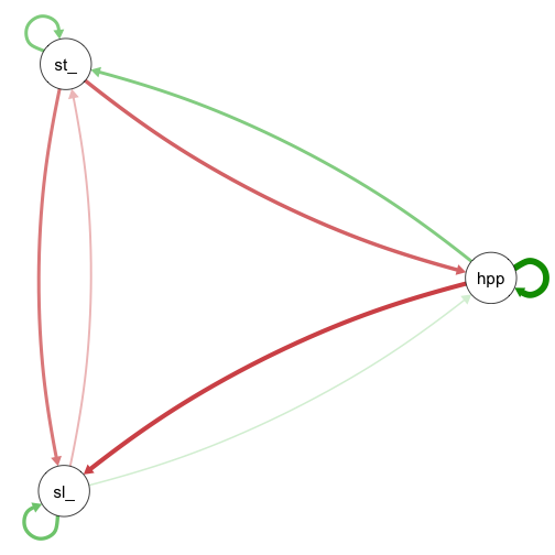
As every other model, the mixed model can be extended by random
effects (Vignette(Random-Effects)), hypothesis tests can be
performed (Vignette(Hypothesis-Testing)).